

Mathematica (9)
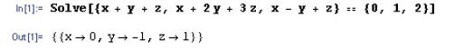
Mathematica can solve systems of linear equations. To
solve the equations
x + y + z = 0, x + 2y + 3z = 1, and x – y + z = 2, we can use the Mathematica
function solve. To do this, make an equation of the list of the left hand sides
of the equations and the list of right hand sides as follows:
Mathematica can also manipulate matrices. To define a matrix, we make a list of lists where the elements of the “outer” list are the columns of the “inner” list of row coefficients. When defining a matrix you must use this format or Mathematica will not know what it is. However, you can display the matrix in standard form, called MatrixForm by using the Mathematica built in function MatrixForm[]. Below are some examples of defining matrices ma and mb, adding, subtracting, and multiplying them, and finding the determinant of ma. (Note that multiplication of matrices uses the period, the same as the dot product of two vectors.)
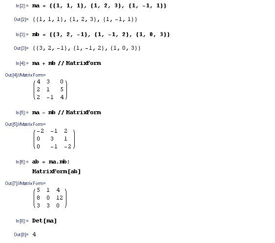
Note that if you don’t want to define a matrix ma + mb
with a special symbol but you still
want to display it in matrix form you can either use MatrixForm[ma + mb] or you
can use the double slash as shown above.
If you want to use matrices to solve a system of linear equations, you write the equations out as ma.mx = mc and the solution is mx = ma-1.mc This is implemented below where the matrix mai is defined as the inverse of matrix ma.
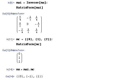
Note that the solutions for x, y, and z are the same 0, -1, and 1 we found above using Solve[].
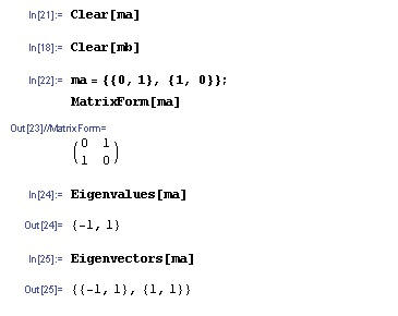
We can also find the eigenvalues and eigenvectors of a square matrix using the Mathematica built in functions Eigenvalues[] and Eigenvectors[]. This is illustrated below. Note that the matrices ma and mb are cleared so they can be redefined although, in this case, mb is not reused.